Rogier

No these data have unfortunately "passed away" with our file server being closed. Which specific files do you need? We might still have them but it will be a manual process.

The coordinates from the original WRF projection are already stored in the west_east and south_north coordinates and the spatial reference is already stored in the crs variable. So to make a tif you can do: import xarray as xr ds = xr.open_dataset("mesoscale-ts.nc") ds_proj_mean = ds.WS.mean("time") ds_proj_mean.rename({"crs":"spatial_ref"}).rio.to_raster("ws_150.tif") That opens it in the right place for me: or to get it in 2157: ds_proj_mean = ds.WS.mean("time") ds_proj_mean = ds_proj_mean.rename({"crs":"spatial_ref"}).drop_vars(["XLAT","XLON"]).rio.reproject("EPSG:2157") ds_proj_mean.rio.to_raster("ws_150_2157.tif")

Hi Lidia, All GWA/WAsP servers were impacted by a major IT issue at DTU. They should now all be working again. Regards

Hi, 1) The new IBZ can also deal with displacement heights in case of forests. It is probably most easy to understand the differences from Fig 1 and 2 in this paper: https://wes.copernicus.org/articles/6/1379/2021/. If you are not using displacement heights the results should be nearly identical, although the new routines also solves some problems with the old routines where "dead pixels" were occurring in the resource grid in some rare cases. You can how to use it here: https://panopto.dtu.dk/Panopto/Pages/Viewer.aspx?id=0394a399-d5c2-4a71-9954-b0d800dbcb7f 2) Yes you can also right click on the GWC now, because that was a more logical place to edit this. You will have to recalculate the GWC after you have changed the heights, because the results will be different. 3) Yes the T* model uses modelled stability parameters from ERA5 to get a overview of sectorwise stability based on the location of the site. It will lookup the nearest ERA5 grid point and retrieve the related stability and boundary layer height. This approach was validated to be better then the old method, see here: https://www.wasp.dk/news/nyhed?id=ea5c4c79-c096-4cc4-a771-ad5314b837ef https://link.springer.com/article/10.1007/s10546-023-00803-3 4) Yes these changes are described here: https://www.wasp.dk/news/nyhed?id=662f23ca-b559-418a-8879-e6b281b7a31f Regards

Yes, there was recently another case that had this problem. The solution there was like this:

There is ways to do that, but I guess the first question is whether you really need a map this big? Usually a distance of about 20 km from yours turbines/mast is more than enough and anything more will not have a significant effect on the flow modelling results, but will make the computations significantly slower.

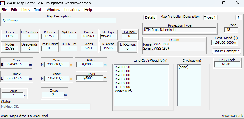
I tried to open your map, but I can see you have used 50 m resolution, so it takes hours to open in the map editor. I would recommend just using the default 100 m resolution, because it will be much faster to open and it will likely make very small differences only for WAsP, which is anyway simplifying the roughness map afterwards. I couldn't detect any errors in the map editor though, see below. Maybe make sure you use the latests version of the map editor and the QGIS plugin?

Yes we recommend always checking with the map editor, but in principle there should be no errors. Could you share your map? Sometimes errors can be solved with "snap geometries to layer" in qgis.

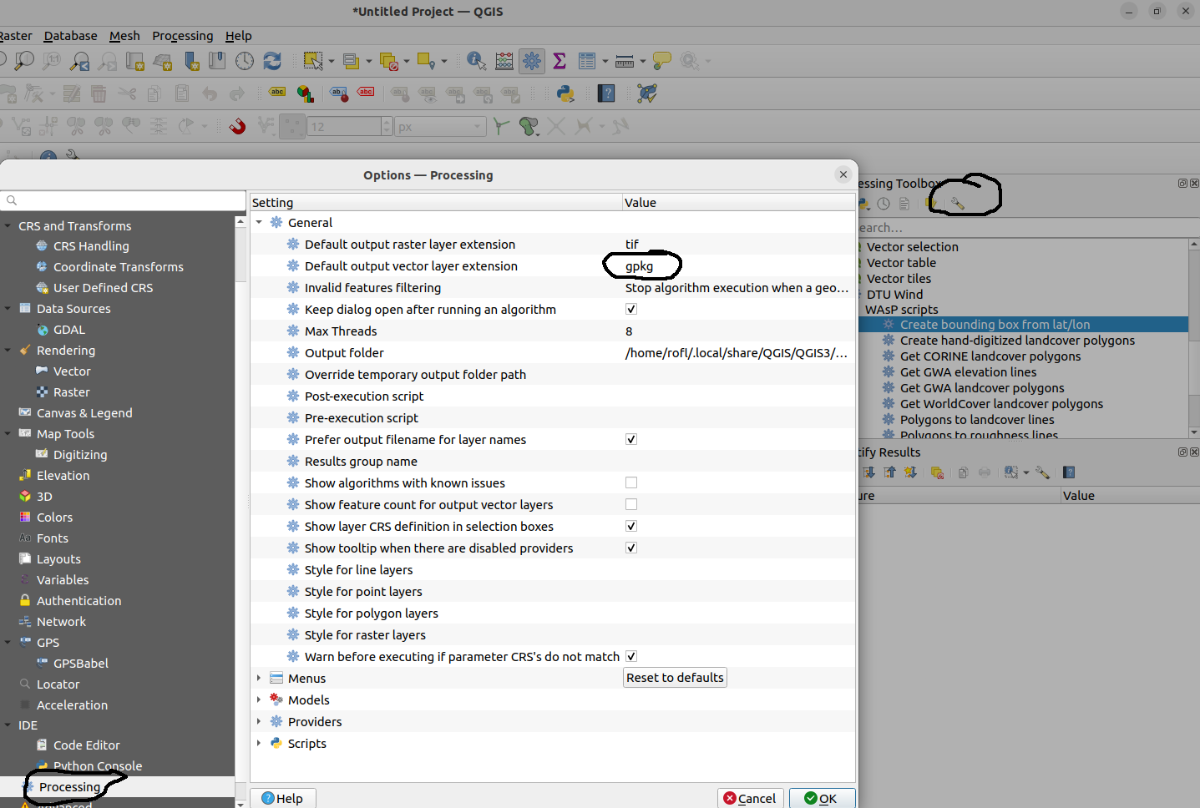
I see, this is a simple bug that I fixed now. The new version will be available soon. This can be when you use the polygonize script in QGIS or other tools. Those scripts don't insert extra nodes where several polygons meet. You can insert those by searching for the script "Snap geometries to layer" and running that. You can also install windkit and use the script poly2lines: https://docs.wasp.dk/windkit/io/topo_autogen/windkit.map_conversion.poly2lines.html

Hi Doha, the papers you mention are indeed the right references. This paragraph in the paper 1 you mention probably explains it best: The original zooming grid is just a grid where the grid cells increase in size further away from the site: The roughness lengths in these cells are then multiplied with a exponentially weighted distance. From those transformed cell values the most significant ones are found with a simple algorithm where you just loop over all roughness changes until you have explained enough of the initial variance in all transformed roughness changes in a certain sector.

Hi Heather, it is not possible yet to do what you describe but we are planning to develop it some time in the future. You can get part of the model chain by applying the speedups but the geostrophic drag law part is currently always converting to histograms (time-independent). If it is just about automating the process you could look at the pywasp or windkit (https://docs.wasp.dk/pywasp/ https://docs.wasp.dk/windkit/) where there is functions to convert from time series to histograms (https://docs.wasp.dk/windkit/io/wc_autogen/windkit.binned_wind_climate.bwc_from_timeseries.html).

I think you can just add the gaps as you want, the significance algorithm is quite robust. Regarding roughness for forest I would for sure not use a standard roughness of 0.5 m. That is generally too low in Europe, where a typical forest has h>10. The rule with z0=h*0.1 will give you usually a much better estimation. The displacement height is automatically calculated since WAsP Release 2022-A-1, if you specifiy them in a .gml file (you can use treeheight *(2/3), see paper I linked before). There is a video about using displacement heights and creating a GML file here: https://panopto.dtu.dk/Panopto/Pages/Viewer.aspx?id=0394a399-d5c2-4a71-9954-b0d800dbcb7f

Yes exactly :)

WAsP CFD (I guess you are talking about the cfdres files) only calculates speedup factors from the terrain. There is no way to get from those files to a wrg file because that format also needs to know the wind distribution (e.g. frequency that the wind is blowing from a certain wind direction sector), which is not present in the cfdres files. So to get from those to the wind resource at 112 m, you will just need to run WAsP itself. That means it does all the steps in the generalization and downscaling of WAsP, using log profile, geostrophic drag law and stability effects. You can read more about those vertical and horizontal extrapolation steps in the European wind atlas and some more recent papers describing the stability model: https://backend.orbit.dtu.dk/ws/portalfiles/portal/112135732/European_Wind_Atlas.pdf https://link.springer.com/article/10.1007/s10546-023-00803-3

These are some good questions and the exact behaviour depends also on WAsP version, as the roughness model has had some changes (mostly version Release 2022-A-1 as described here: https://www.wasp.dk/download/wasp12_releasenotes) If you are using WAsP from that version onwards it generates a zooming grid as a first step of processing a vector map. This is called spider grid analysis in this paper: https://wes.copernicus.org/articles/6/1379/2021/wes-6-1379-2021.html you can read more about how it works. It is probably most useful to look at Fig 2 there, which shows the spider grid analysis with the roughness lengths in all cells (2b) and the reduced number of roughness changes that is indeed 10 as you describe (2c). This is just to say that if there is a very small gap between polygons it will be aggregated anyway within a cell and it will not necessarily count as a change, because first a log averaged z0 weighted by landcover class areas in a cell is calculated. I copy the relevant part about the roughness reduction algorithm from this paper: https://wes.copernicus.org/articles/3/353/2018/wes-3-353-2018.pdf So in summary the both the distance to the roughness change and the change itself are important for the algorithm that selects the most significant roughness changes. It does not filter from the site outwards and stops when it has found 10 as you seem to think. It looks at all roughness cells simultaneously and also takes into account the distance to change. To some extent it can be problematic to have high-resolution maps of forested sites, because the few pixels with low roughness will lower the aggregated roughness quite a lot for WAsP (see Fig. 8 of the last mentioned paper), while in reality these pixels might even increase the effective roughness of a area due to additional form drag. For those cases it might make sense to use a higher roughness length then you would expect to alleviate this problem. But this is a different issue from which you are talking about, I think.